By Octavio Medina @octavio_medina
Wait times matter. They are frustrating, they make it harder to access critical services, and they waste people’s time. What’s more, wait times also disproportionately impact the low-income population, which spends significantly more time lining up in queues. For example, The Economist recently ran an article that used some American Time Use Survey data to suggest that those making under $20,000 a year have to wait 46 minutes a day for public services, whereas the figure for those making over $150,000 is 12 minutes less. It may not sound like much, but that’s ten full working days a year! If we take the NYC area median income ($86,000 a year), then 10 days of work per year means that lower income folks "pay" more than $3,000 per year in extra lost working hours. This is important because low-income households already face chronic resource scarcity.
Fortunately, many businesses and public agencies have started paying attention to the huge costs of waiting. More and more agencies routinely measure (and publicly share) their wait time metrics. For example, NYC has been publishing average wait times for Job Centers and SNAP field offices for quite some time now. Measuring wait times is a good start, because at least it makes a problem visible.
Today, I’ll talk about a phenomenon that’s relevant to wait times, but remains fairly unknown: the inspection paradox.
The inspection paradox
Have you ever called customer service only to find that they’re experiencing higher than normal call volumes? In fact, does this seem to happen all the time? Or have you ever felt that subway cars, airplanes, or buses are always crowded, while the transit authority or airline says the system is under-utilized?
You may be tempted to come up with reasons for this: perhaps longer or more crowded train rides are more salient, or they’re just more available in our memory because they make us angry; the same could be possible for customer service experiences. Or perhaps the transit authority or business is just wrong about the metrics they’re using.
And the short answer is that both you and the transit authority may very well be right, you’re just looking at things from a slightly different perspective. The explanation is what Allen Downey calls the inspection paradox. Here’s an example of this phenomenon in action:
"Suppose you ask college students how big their classes are and average the responses. The result might be 90. But if you ask the college for the average class size, they might say 35. It sounds like someone is lying, but they could both be right."
"When you survey students, you oversample large classes: If there are 10 students in a class, you have 10 chances to sample that class; if there are 100 students, you have 100 chances. In general, if the class size is x, it will be overrepresented in the sample by a factor of x."
How does this apply to customer service, airplanes, and waiting times? When an airplane is almost empty, very few people are there to see it (and enjoy it!). But when an airplane is crowded and uncomfortable, by definition there are more witnesses. So from a customer’s perspective, the service is worse. But that doesn’t mean the airline’s numbers are wrong. It’s just that if you’re randomly sampling a passenger, you’re far more likely to pick one that traveled in a busy flight, but if you’re randomly sampling a plane, you may very well pick one that’s basically empty.
As Downey says, once you learn about this phenomenon, you start seeing it everywhere (if this interests you, Downey gave an excellent talk a couple of years ago where he discussed this at length).
One of the places where it pops up is wait times. On days where the Job Center or DMV has a very short wait time, it’s likely because there aren’t that many customers around–which means few people get to enjoy it. And on long wait time days, the opposite is true.
But don’t take my word for it. Let’s take a look at the Customs and Border Protection Bureau’s data on wait times across American airports. Let’s use data for JFK from July 2018 to July 2019. We have hourly wait time figures for a bunch of terminals, as well as totals, and breakdowns by nationality. The source file is available here. You can follow along with the R code below (but feel free to jump to the graph).
First, we read in the data and clean some of the variables. Then we calculate two different metrics. The first is the average wait time from the perspective of the airport: what’s the average hourly wait time as observed by CBP officers? The second average tries to answer this question from the perspective of the customers: what was the average hourly wait time as experienced by a passenger crossing the border? We do this by weighting the average using the total number of passengers processed (total).
library(tidyverse)
library(hrbrthemes)
library(wesanderson)

jfk_raw <- read_csv("https://raw.githubusercontent.com/ideas42/data42/main/jfk.csv")

jfk <- jfk_raw %>%
  janitor::clean_names()


t <- jfk %>%
  group_by(terminal) %>%
  summarize(mean_wait = mean(wait_all),
            mean_wait_weighted = weighted.mean(w = total, wait_all),
            ratio = mean_wait_weighted / mean_wait)
The graph below shows the results, and there are interesting patterns across the board. Unsurprisingly, wait times are much shorter late at night, because there are fewer arrivals. Wait times peak during the early afternoon, and then dip again until later in the evening. But to our point, note that for every single hour of the day, the passenger-weighted wait time is higher than the simple average wait time. This time we already know why: most passengers arrive when wait times are longer. That’s why it’s busy in the first place!
t_long <- t %>%
  rename(Airport = mean_wait,
         Passenger = mean_wait_weighted,
         Hour = hour) %>%
  pivot_longer(names_to = "Metric", values_to = "Wait", Airport:Passenger)

t_long %>%
  ggplot(aes(Hour, Wait, color = Metric, group = Metric)) +
  geom_point() +
  geom_line() +
  theme_ipsum_ps() +
  scale_color_manual(values = wes_palette("Darjeeling1")) +
  labs(title = "Average Hourly Wait Time - JFK (July 2018 - July 2019)",
      x = "Time of Day",
      y = "Wait (Minutes)") +
  scale_x_discrete(guide = guide_axis(n.dodge = 2))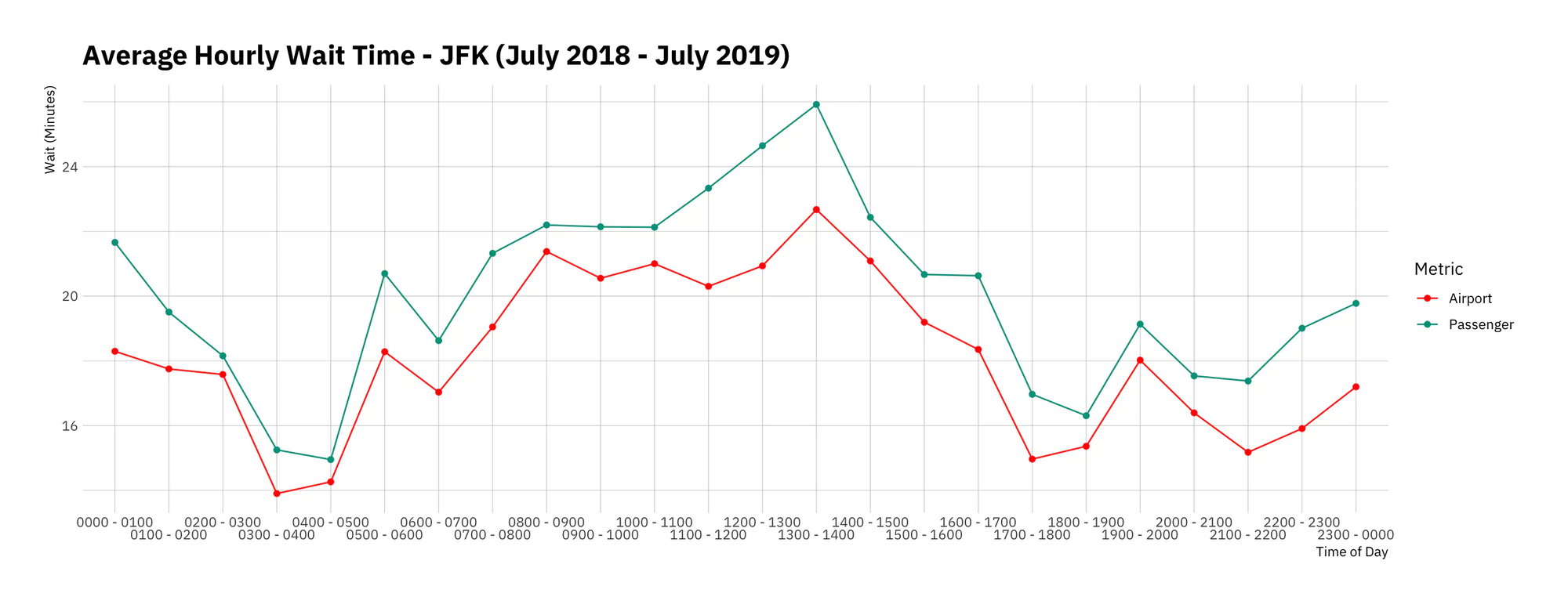
While in our example the differences aren’t huge (all of them are under 10 minutes), this is not always the case. That’s why it’s crucial to be aware of what exactly you’re measuring, and from whose perspective. In recent years, the cost of collecting data has fallen tremendously; as a result, more and more organizations are routinely doing it. But collecting more data alone does not tell you how to improve decision-making or make services better. For that, you need both human judgment and qualitative data.
At ideas42 we like to think that this mix of judgment and user research can help enrich and explain our quantitative work. Going out, observing the context, and talking to people who are embedded in it can allow you to gain insights that would otherwise be unavailable. Of course, the reverse is also true: data analysis and number-crunching almost always help augment any insights gained from observation or interviews.
In Part II we’ll talk about a separate metric that’s relevant for wait times: variance.